Chapter 1: An activity with rules in which people or teams compete against each other
A simulation of how the shape of our social ties, and the way rewards are counted, decide if and when we cooperate
Published
November 8, 2026
It’s not really news if you knew that I have strong opinions against the current models of social media platforms. The current model which relies on the commercialisation of attention and virality is simply unethical in my opinion. I have been avoiding using any kind of social media for a few years now, just for the sake of my own sanity.
Recently, as I was combatting the urge to engage with these platforms, so I decided to just play some video games, I used to love it when I was younger. I would go every Sunday to an internet shop and play for 2 hours over the intranet of the store with whoever is in there. Half-Life and Counter-Strike were so fun, FIFA 2007 was amazing, and PES 2013 was legendary.
Those memories inspired me to write (in the future) about games, and the political economy of the current model of social media. Then, as I side quested to redesign this website and showcase my previous work, I realised as I struggled with different decisions, that maybe I should write about that: How decisions are made. Given my struggles, the prisoner’s dilemma as a project subject was a perfect sub-sub-side-quest.
So, to cut the yapping short, the objective of this post is to explore the idea of the prisoner’s dilemma, starting from the simplest example of a 2-player game, then building complexity throughout to generalise the concept to a multiplayer game.
The prisoner’s dilemma is a simple puzzle, but it provides us with powerful insights into human behaviour when we assume rationality. The puzzle in its simplest form is as follows: two players meet, they have to choose, without knowing each other’s decision preference beforehand, whether to cooperate with the other player, or to defect from cooperating. What governs the decision is the reward rules determined by:
Temptation (T): the payoff of defecting.
Reward (R): the payoff of cooperating.
Punishment (P): the payoff of mutual defection.
Sucker’s pay-off (S): the payoff of being exploited (one player cooperates, the other defects)
Essentially, a game with these rules such that:
\[T > R > P \ge S\]
is considered a form of the prisoner’s dilemma. The pay-off possibilities for a 2-player game can be summarised in this table below:
We’ll build the answer in small steps: first two players and one choice, then a crowd of players who copy each other, and finally players living in networks of different shapes.
Cheating is tempting
In this game as we set it up, we assume that neither player knows what the other would decide. They would have to rationalise their decision in a way that matches their preferences. Maybe a player would want to get as many points as possible, another may want to avoid risks and not lose instead.
But in this game, there’s only one strategy that both minimises risk and maximises potential gains. We can identify this strategy if we completely ignore what the other player does and focus mainly on the range of payoffs we can get from each of the decisions ahead. In other terms if we sum the payoffs row-wise we get the total payoff of each decision.
In here, because the relationship \(T > R > P \ge S\) is satisfied, the only winning strategy is to defect. Because the total payoff of defecting is higher than cooperating. It’s tempting to cheat, or in this case betray the other. How Machiavellian.
Now you may ask this is basic logic, why is this a big deal, where’s the dilemma? The answer simply put is that a careful, self-interested (rational) player would decide to defect. The other player reasons in exactly the same way, so both defect and both earn 0, while cooperating would have given each of them 1.
More specifically, the dilemma here is that what is rational for each player is bad for both. A classic example I’d like to use in class to explain two paradoxical ideas, that both individualism and central coordination result in sub-optimal results for the individual and the group, someone will have to lose eventually.
Dominant strategy. A choice that is at least as good as any alternative, whatever the others do. Here, defecting.
Nash equilibrium. A situation where no player can do better by changing only their own choice. Here, both defecting: a player who switches to cooperating alone still earns 0, so gains nothing.
Extending the game to many players
So far in a game with two players, both end up reasoning their way to defecting. However, in reality, people socialise with more than just one peer, and their interactions influence each other’s behaviour at least to some extent.
We can extend our game into the multi-player set up, simply by imposing a very simplistic assumption about how players decide, they will compare their outcome to the outcome of their peers, and copy the strategy that got the best payoff.
To establish this game and discover how the behavior of its players evolves in each round. In here I will go for 300 rounds with 100 players, and the initial game will dictate the proportion of defectors and cooperators that’s assigned to the players at random, then we will tweak what we mean by peers or neighbours. Essentially we will control the number of comparisons each player does. This will require further elaboration that I will go through here and explain how to implement it in R.
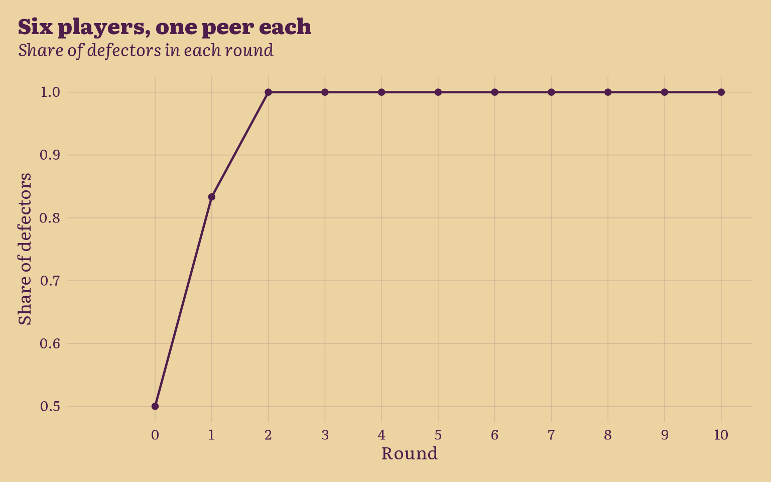
Let’s start with a simple case of 6 players, each player will have one peer. This is a simple social network that we can visualise considering a player as a node, with an edge linking it to its peer. We will first assign randomly the decision of each player for the initial game then see what happens after 36 games.
Show the code
players <-1:6rounds <-1:36peer <-sample(players, replace = F)peers <-tibble(player = players,peer = peer)# random assignment of the initial decision, # function of x the proportion of defectorsinitial_decision <-sample(rep(c("cooperate", "defect"), each =length(players) /2))## turn the payoff rule into a functionpayoff_rule <-function(decision_player, decision_peer){case_when( decision_player =="cooperate"& decision_peer =="cooperate"~1, # R decision_player =="cooperate"& decision_peer =="defect"~-1, # S decision_player =="defect"& decision_peer =="cooperate"~1.2, # T decision_player =="defect"& decision_peer =="defect"~0, # PTRUE~NA_real_ )}df0 <- peers |>mutate(round =0,decision_player = initial_decision,decision_peer = decision_player[peer] ) |>mutate(payoff_player =payoff_rule(decision_player, decision_peer),payoff_peer =payoff_rule(decision_peer, decision_player) )
Now, this is the initial state of the game, from here, we want to move to the next rounds, each player will look at their neighbour and compare their payoffs, if the difference favors the peer, the player will copy its peer, otherwise it will continue with its winning strategy. To implement this we need a bit of engineering so bear with me.
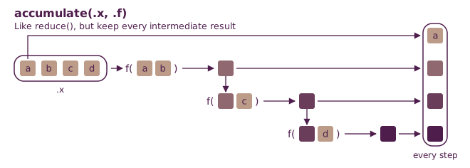
The objective here is to move from the initial state to next rounds, the payoff of each previous round is the input for the decision in the next. This is a perfect case for map/reduce functions. These are, in R, vectorised and fast family of functions that replace loops and are extremely efficient. These functions are part of the purrr package, probably my favorite. In here I will use a variant of the reduce family called accumulate.
Diagram adapted from the purrr cheatsheet by Posit Software, PBC (CC BY-SA 4.0).
All we have to do is apply the same logic in each round
Okay, now we should see this clearly in a graph. I will calculate the proportion of defectors in each round. But what can we expect here? From what we’ve already seen, players will quickly realise that defecting is a better strategy and eventually all six players will defect and remain so.
Show the code
final |>mutate(decision =if_else(decision_player =="defect", 1, 0) ) |>summarise(defectors =mean(decision), .by = round ) |>ggplot() +geom_line(aes(x = round, y = defectors ) ) +geom_point(aes(x = round, y = defectors ) ) +scale_x_continuous(limits =c(-1, 10), breaks =seq(0, 10, by =1)) +labs(title ="Six players, one peer each",subtitle ="Share of defectors in each round",x ="Round",y ="Share of defectors" ) +theme_bmh()
Now, there are different moving parts in here. We can manipulate the initial conditions of the game to explore how the proportion of players adopting the dominant strategy changes. We can increase the number of players, of rounds, and we can change the initial proportions of defectors.
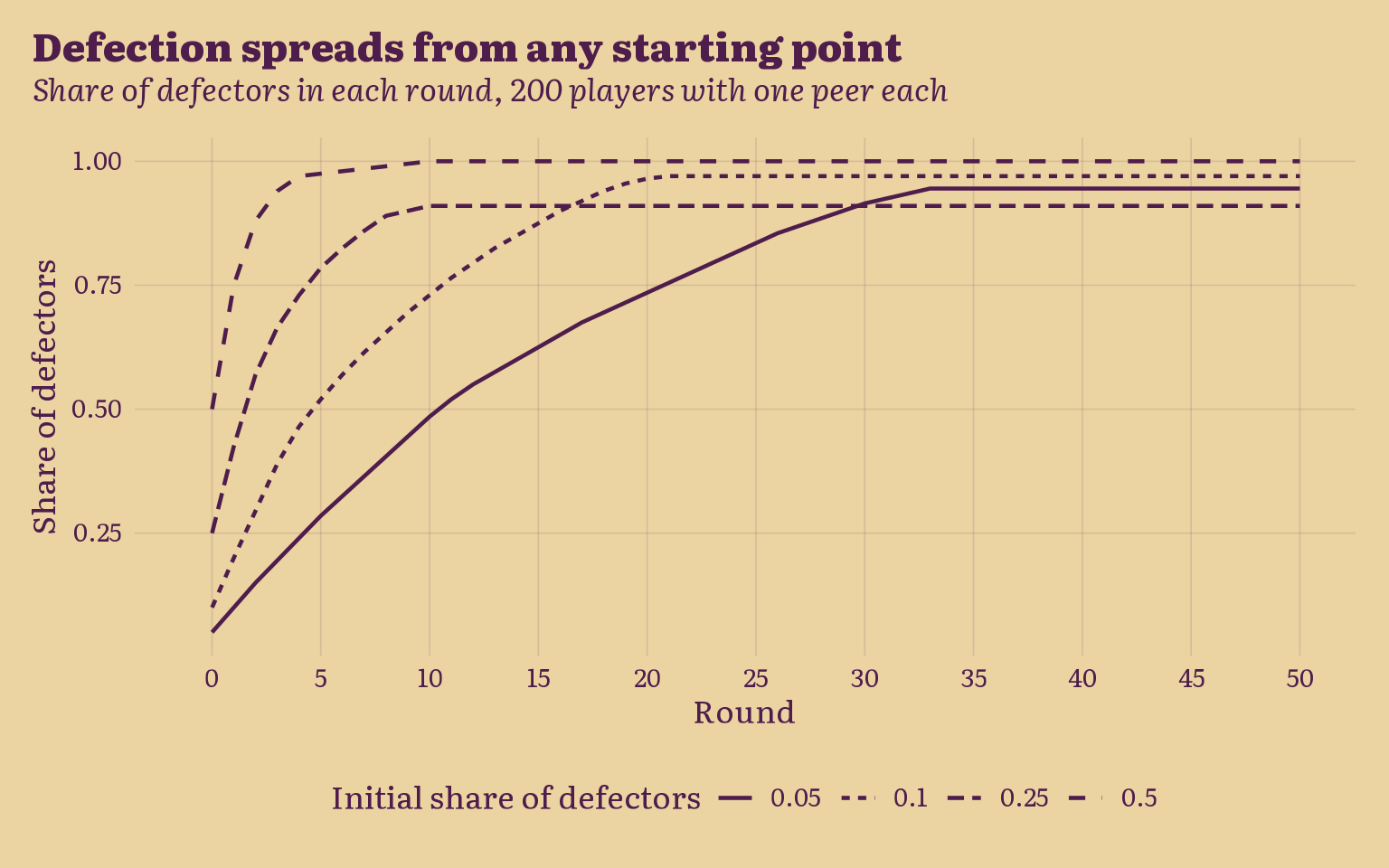
For convenience, let’s see what happens when we have a large group of players, with one single defector. If you expect the same result to happen, everyone eventually defects but after more rounds, you are on the right track. However, since I’m lazy, I don’t want to rewrite all the code again or even copy paste it. So I’m simply going to turn it into a function that controls for the number of players, the proportion of defectors and the number of rounds.
init_cond <-c(0.05, 0.1, 0.25, 0.5)sims <-map( init_cond,~simulate_game(prop_defect = .x))all_sims <-map2(.x = init_cond,.y = sims,~ .y |>mutate(initial_proportion =as.factor(.x)) ) |>bind_rows()all_sims |>mutate(decision =if_else(decision_player =="defect", 1, 0) ) |>summarise(defectors =mean(decision), .by =c(round, initial_proportion) ) |>ggplot() +geom_line(aes(x = round, y = defectors,linetype = initial_proportion ) ) +scale_x_continuous(limits =c(-1, 50), breaks =seq(0, 50, by =5)) +labs(title ="Defection spreads from any starting point",subtitle ="Share of defectors in each round, 200 players with one peer each",x ="Round",y ="Share of defectors",linetype ="Initial share of defectors" ) +theme_bmh()
Great, we have successfully generalised the game to many players that play each round with their peers. Still, we can improve this simulation to many other real life conditions. For instance, usually people have multiple peers, and they make mistakes, they can misjudge the success of their peer’s strategy. There are different patterns of social interactions, close group of friends, friends centered around one leader, and people who are friends with many groups at the same time. All of these granularities compound the complexity of the simulation, and show us different outcomes for different social architectures.
Now, how can we implement these ideas? The simplest answer is usually formal and mathematical. But I will not get into too much details unless we really need to. So I will try to decipher this into the most basic ideas first, starting from the different patterns of interaction between people, to the idea of mistakes or uncertainty.
The reason why I chose to write this post in this way is because it sits at the intersection of concepts that really interest me. Networks, probabilities, games, and simulations. We started this post with the simplest game, then extended the game to many players, we simulated it and showed that even when we have a very small number of defectors, everyone will eventually choose to copy the dominant strategy and defect.
To extend this further, I want to discuss different patterns of social networks. These patterns are very interesting because they inform us on how people interact, and that also changes the way the game evolves. You would be right to assume that eventually all players defect.
But before we get into the details let’s reason our way through this. Usually, there are two questions that determine the patterns of interactions between people in a community.
How many friends does the typical person have?
Do my friends know each other?
From these two questions, we can build distributions of connections. In this version we want to have a more realistic description of how people interact. Albeit realistic here is a bit of a stretch, because I will still use simulated data. There’s a wealth of actual network data sets on the web, but I want to practice simulating data more through this. You are stuck with my side quest this time.
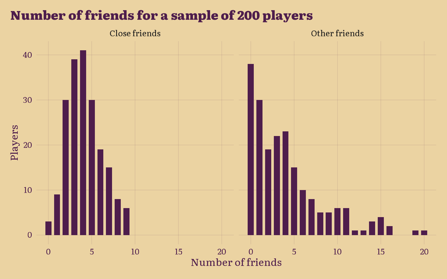
Let’s start with an example, one person. How can we model the relationship of a typical person? Well, since the number of friends is essentially a count we can rely on the Poisson distribution for that. For the non-close friends, the negative binomial is a better fit. Let’s see how a sample of 200 players would look like if we assume that the average count of close friends is 4, and the other acquaintances is 2.
Show the code
n <-200close <-rpois(n = n, lambda =4)others <-rnbinom(n = n, size =1, mu =4)friends <-tibble(player =1:n, close = close,others = others)friends |>pivot_longer(c(close, others), names_to ="type", values_to ="friends") |>mutate(type =if_else(type =="close", "Close friends", "Other friends")) |>ggplot(aes(friends)) +geom_bar(fill = palette$ink, width =0.7) +facet_wrap(~ type) +labs(# title = "Close friends and other friends",title ="Number of friends for a sample of 200 players",x ="Number of friends",y ="Players" ) +theme_bmh()
Now, we can move forward and build our network of players. We will do the same thing as the previous version, only this time, each player has different peers to play the game with and the number of these peers is sampled from the distributions above. However, notice that the distributions actually inform us on the size of the friends groups and acquaintances. So in order to build the network we should start from there. First we will generate some groups of friends whose size is sampled from the Poisson, all these friends are peers to each other. Then we will assign another number of peers from other non group members randomly sampled from the negative binomial distribution.
Show the code
groups <-tibble(player =1:n) |>mutate(group =rep(seq_len(n), times =1+rpois(n, 3))[player] )close <- groups |>inner_join( groups |>rename(friend = player), by ="group", relationship ="many-to-many" ) |>filter(player != friend) |>select(player, friend)# 2. Other friends: one ticket per friendship a player wants, shuffled and paired two by twoother <-tibble(player =1:n, n_other =rnbinom(n, mu =2, size =1) ) |>uncount(n_other) |># one row per ticketslice_sample(prop =1) |># shuffle the ticketsmutate(pair =ceiling(row_number() /2)) |># tickets 1-2, 3-4, ... form pairsfilter(n() ==2, .by = pair) |># drop a leftover ticketsummarise(friend =last(player), player =first(player), .by = pair) |>filter(player != friend) |>select(player, friend)# For the game: every friendship in both directions, no duplicatesfriendships <-bind_rows( close |>mutate(type ="close"), other |>mutate(type ="other"), other |>select(player = friend, friend = player) |>mutate(type ="other")) |>distinct(player, friend, .keep_all =TRUE) |>rename(peer = friend)
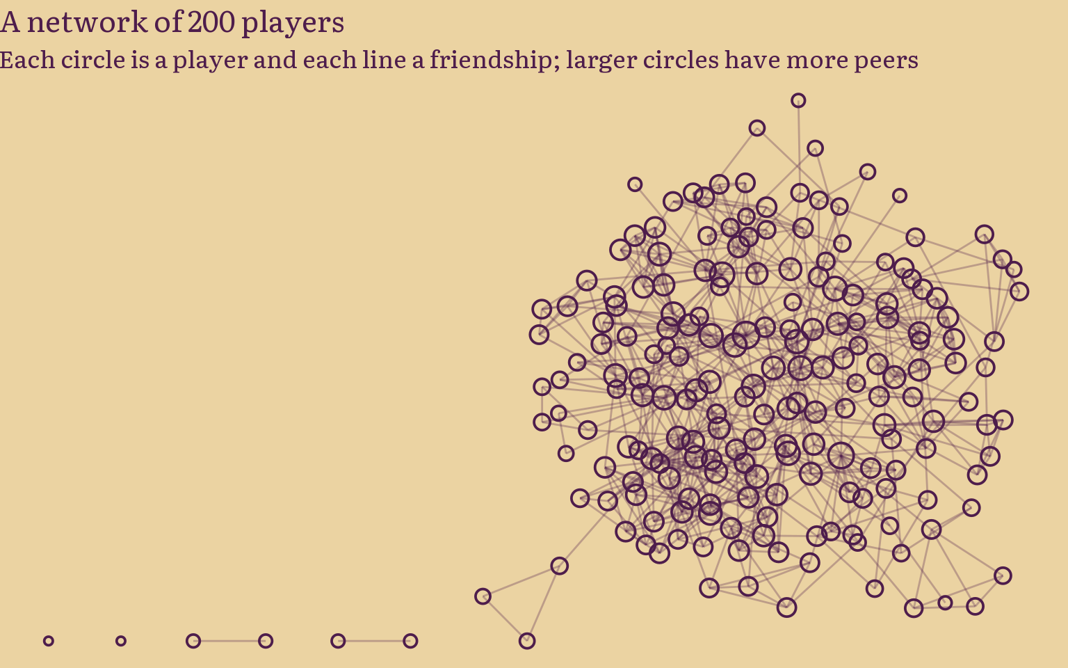
Let’s visualise how the new network looks like:
Show the code
friends_network <-tbl_graph(nodes =tibble(player =1:n),edges = friendships |>filter(player < peer) |>select(from = player, to = peer, type),directed =FALSE) |>mutate(deg =centrality_degree())friends_network |>ggraph() +geom_edge_link(colour =alpha(palette$ink, 0.3)) +geom_node_point(aes(size = deg),shape =21,colour = palette$ink,stroke =1 ) +scale_size(range =c(1.5, 6), guide ="none") +# scale_fill_manual(values = c(cooperate = "#3b7dd8", defect = "#d8574a")) +labs(title ="A network of 200 players",subtitle ="Each circle is a player and each line a friendship; larger circles have more peers" ) +theme_bmh_void()
Using "stress" as default layout
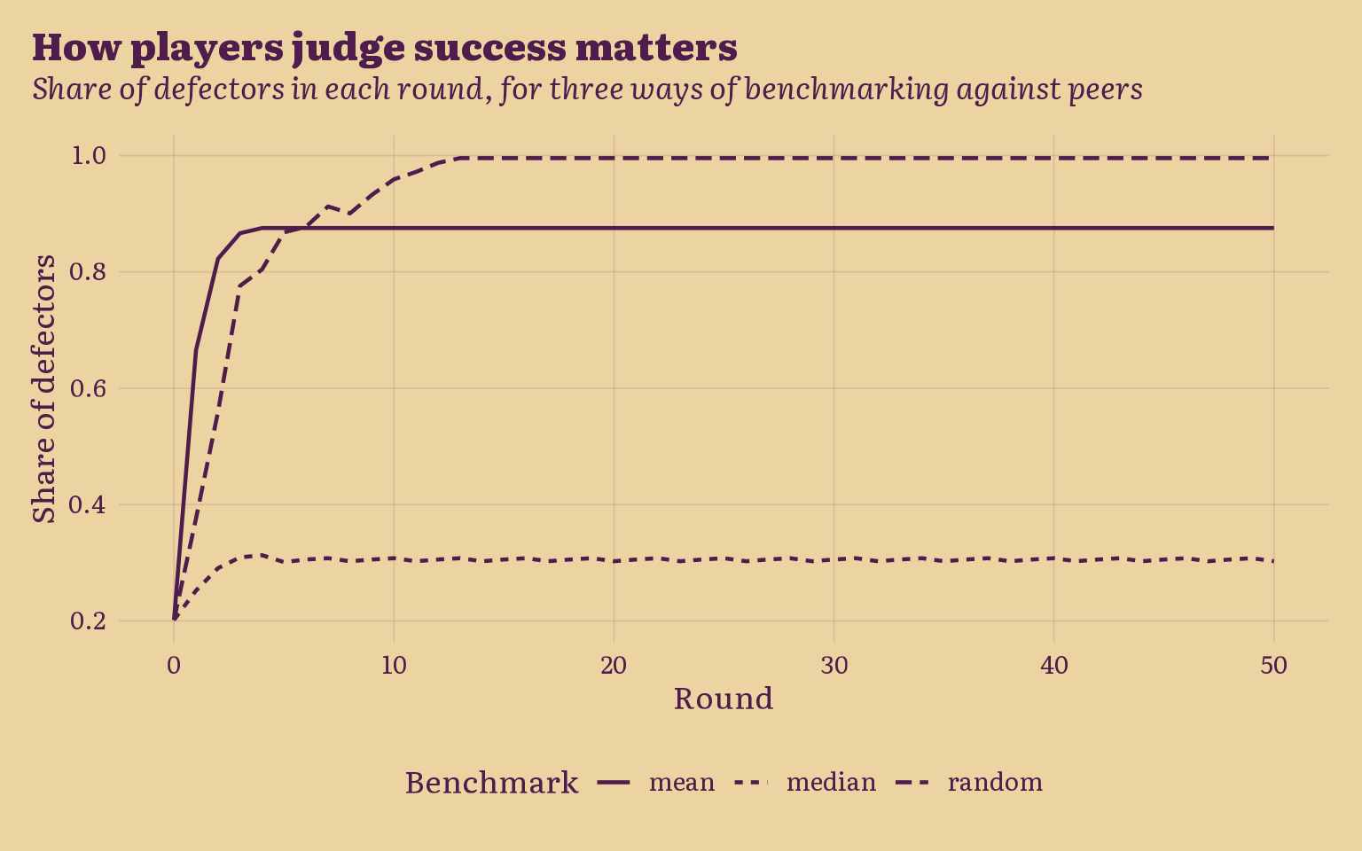
We can now run the experiment again, the only difference here is that instead of player comparing its payoff to one peer, it will do so with all its peers instead. So we need to specify what number the player is going to use as benchmark. We can see the average, the median, or we can choose a random peer. Let’s do all three.
Show the code
# ---- 1. Assign peers from the two distributions ----assign_peers <-function(n_players) { players <-seq_len(n_players)# close friends: groups of 1 + Poisson(3) players, all peers to each other groups <-tibble(player = players) |>mutate(group =rep(players, times =1+rpois(n_players, 3))[player]) close <- groups |>inner_join(rename(groups, peer = player), by ="group", relationship ="many-to-many") |>filter(player != peer) |>select(player, peer)# other friends: tickets from the negative binomial, shuffled and paired other <-tibble(player = players, n_other =rnbinom(n_players, mu =3, size =1)) |>uncount(n_other) |>slice_sample(prop =1) |>mutate(pair =ceiling(row_number() /2)) |>filter(n() ==2, .by = pair) |>summarise(peer =last(player), player =first(player), .by = pair) |>filter(player != peer) |>select(player, peer)# every friendship in both directions, without duplicatesbind_rows( close |>mutate(type ="close"), other |>mutate(type ="other"), other |>select(player = peer, peer = player) |>mutate(type ="other") ) |>distinct(player, peer, .keep_all =TRUE)}# ---- 2. Every player plays the game with every peer ----play_peers <-function(peers, decisions) { peers |>left_join(decisions, by ="player") |>left_join(rename(decisions, peer = player, decision_peer = decision_player), by ="peer") |>mutate(payoff_player =payoff_rule(decision_player, decision_peer),payoff_peer =payoff_rule(decision_peer, decision_player) )}# ---- 3. One rule for scores and benchmarks ----score_rule <-function(payoff, rule) {if (rule =="median") median(payoff) elsemean(payoff)}# ---- 4. One round: score, compare, copy, play again ----play_round_peers <-function(df, rule ="mean") {# each player's score: their payoffs, summarised by the rule scores <- df |>summarise(score_player =score_rule(payoff_player, rule), .by = player)# each row also gets the peer's score compared <- df |>left_join(scores, by ="player") |>left_join(rename(scores, peer = player, score_peer = score_player), by ="peer")# the random rule looks at a single peer, as in the one-peer gameif (rule =="random") compared <-slice_sample(compared, n =1, by = player)# benchmark from the peers' scores, with the same rule; remember the best peer switches <- compared |>summarise(benchmark =score_rule(score_peer, rule),score_player =first(score_player),decision_best = decision_peer[which.max(score_peer)],.by = player ) |>filter(benchmark > score_player) |>select(player, decision_best)# new decisions: copy the best peer if the peers did better decisions <- df |>distinct(player, decision_player) |>left_join(switches, by ="player") |>mutate(decision_player =coalesce(decision_best, decision_player)) |>select(player, decision_player)# play the next round with the new decisionsplay_peers(select(df, player, peer, type), decisions) |>mutate(round = df$round[1] +1)}# ---- 5. Main simulator ----simulate_game_peers <-function(n_players =200,prop_defect =0.01,n_rounds =300,rule ="mean",seed =NULL) {if (!is.null(seed)) set.seed(seed)# 1. Peers from the two distributions peers <-assign_peers(n_players)# 2. Initial decisions with a controlled proportion of defectors n_defect <-round(n_players * prop_defect) n_coop <- n_players - n_defect decisions <-tibble(player =seq_len(n_players),decision_player =sample(c(rep("cooperate", n_coop), rep("defect", n_defect))) )# 3. Round-0 state df0 <-play_peers(peers, decisions) |>mutate(round =0)# 4. Iterate history <-accumulate(seq_len(n_rounds), ~play_round_peers(.x, rule), .init = df0)bind_rows(history)}rules <-c("mean", "median", "random")# init <- c(0.1, 0.25, 0.5)all_sims_peers <-map( rules,~simulate_game_peers(n_players =200,prop_defect =0.2,n_rounds =50,rule = .x,seed =2) |>mutate(rule = .x)) |>bind_rows()all_sims_peers |># distinct(round, rule, player, decision_player) |> # one row per player per roundmutate(decision =if_else(decision_player =="defect", 1, 0) ) |>summarise(defectors =mean(decision),.by =c(round, rule) ) |>ggplot() +geom_line(aes(x = round,y = defectors,linetype = rule,# colour = shades(init) ) ) +# facet_grid(~ init) +# scale_x_continuous(limits = c(-1, 50), breaks = seq(0, 50, by = 5)) +labs(title ="How players judge success matters",subtitle ="Share of defectors in each round, for three ways of benchmarking against peers",x ="Round",y ="Share of defectors",linetype ="Benchmark" ) +theme_bmh()
Aha, now this plot is interesting. But before we go through with this, let me explain what’s happening behind the scenes. The most important part here is the benchmarking process. A player would play as many games as they have peers each round, then they will benchmark their payoff against them. How the player aggregates that information influences their decision. When players pick a random peer to compare with, eventually all players defect after 12 games. However this doesn’t hold when players start benchmarking in aggregates. When players compare their average payoff, with averages of their peers, they start adopting the dominant strategy faster than the random benchmark, but unlike the latter, the proportion of the players that adopt the strategy saturates at around 90% very early on and remains in that steady state. But the story changes completely when player consider the median instead. When they consider the half point payoff of their games with their peers, the adoption of the dominant strategy saturates at around 30%. What we can say here is that, collaboration as a strategy survives even relatively even when it’s not the dominant strategy when the social ties between players are strong.